Tutorial on pyfastnoisesimd usage
Workflow
The basic workflow of using pyfastnoiseimd (which we will refer to as fns) is:
Instantiate a noise object as:
noiseObj = fns.Noise()
Set the desired properties of the noiseObj using some recipe of values. The precise recipe used is where noise generation morphs from mathematics to an artistic endeavor. One big advantage of using Python in this instance is that it becomes easy to quickly prototype many different styles of noise and adjust parameters to taste.
Use either fns.Noise.genAsCoords() to generate 1-3D rectilinear noise or fns.Noise.genFromCoords() to generate noise at user-generated coordinates. The fns.Noise class is a mapping of Python properties to the set<…> functions of the underlying FastNoiseSIMD library. Please see the API reference for the properties that may be set.
The fns.Noise class contains three sub-objects:
- Noise.cell: contains properties related to cellular (cubic Voronoi) noise.
- Noise.perturb: contains properties related to perturbation of noise, typically related to applying gradients to noise.
- Noise.fractal: contains properties related fractal noise. Fractals layer noise of similar properties but log-scaled frequencies (octaves).
Example with source
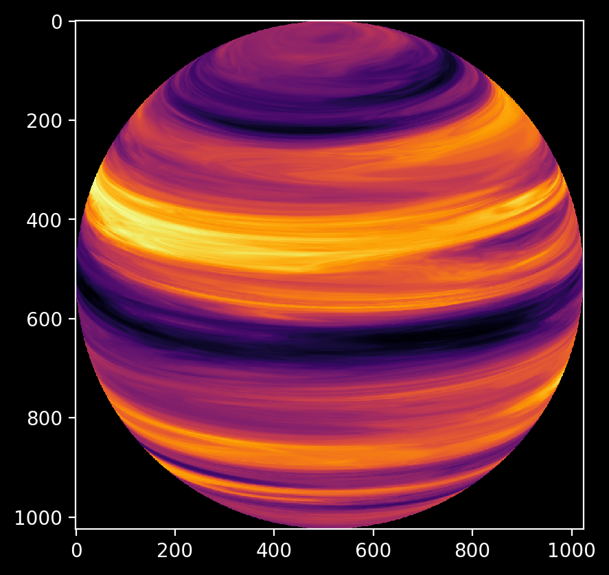
In this case, we want to simulate a height-map on the surface of a sphere, and project coordinates from a 2D orthographic projection (i.e. a sprite) to the 3D Cartesian coordinates that FastNoiseSIMD requires, generate the noise, and then return back to the coordinates of our computer monitor.
The mathematics for the projection can be found at:
https://en.wikipedia.org/wiki/Orthographic_projection_in_cartography
Here is an example output using a recipe
Here is the complete source code:
import numpy as np
from time import perf_counter
import pyfastnoisesimd as fns

import matplotlib.pyplot as plt
plt.style.use('dark_background')
from mpl_toolkits.mplot3d import Axes3D

def orthoProject(noise:fns.Noise, tile2: int=512, p0: float=0., l0: float=0.) -> np.ndarray:
    '''
    Render noise onto a spherical surface with an Orthographic projection.

    Args:
        noise: a `pyfastnoisesimd.Noise` object.
        tile2: the half-width of the returned array, i.e. return will have shape ``(2*tile2, 2*tile2)``.
        p0: the central parallel (i.e. latitude)
        l0: the central meridian (i.e. longitude)

    See also:

        https://en.wikipedia.org/wiki/Orthographic_projection_in_cartography

    '''
    # We use angular coordinates as there's a lot of trig identities and we
    # can make some simplifications this way.
    xVect = np.linspace(-0.5*np.pi, 0.5*np.pi, 2*tile2, endpoint=True).astype('float32')
    xMesh, yMesh = np.meshgrid(xVect, xVect)
    p0 = np.float32(p0)
    l0 = np.float32(l0)

    # Our edges are a little sharp, one could make an edge filter from the mask
    # mask = xMesh*xMesh + yMesh*yMesh <= 0.25*np.pi*np.pi
    # plt.figure()
    # plt.imshow(mask)
    # plt.title('Mask')

    # Check an array of coordinates that are inside the disk-mask
    valids = np.argwhere(xMesh*xMesh + yMesh*yMesh <= 0.25*np.pi*np.pi)
    xMasked = xMesh[valids[:,0], valids[:,1]]
    yMasked = yMesh[valids[:,0], valids[:,1]]
    maskLen = xMasked.size

    # These are simplified equations from the linked Wikipedia article.  We
    # have to back project from 2D map coordinates [Y,X] to Cartesian 3D
    # noise coordinates [W,V,U]
    # TODO: one could accelerate these calculations with `numexpr` or `numba`
    one = np.float32(0.25*np.pi*np.pi)
    rhoStar = np.sqrt(one - xMasked*xMasked - yMasked*yMasked)
    muStar =  yMasked*np.cos(p0) + rhoStar*np.sin(p0)
    conjMuStar = rhoStar*np.cos(p0) - yMasked*np.sin(p0)
    alphaStar = l0 + np.arctan2(xMasked, conjMuStar)
    sqrtM1MuStar2 = np.sqrt(one - muStar*muStar)

    # Ask fastnoisesimd for a properly-shaped array
    # Failure to use a coords array that is evenly divisible by the
    # SIMD vector length can cause a general protection fault.
    coords = fns.empty_coords(maskLen)
    coords[0,:maskLen] = muStar                             # W
    coords[1,:maskLen] = sqrtM1MuStar2 * np.sin(alphaStar)  # V
    coords[2,:maskLen] = sqrtM1MuStar2 * np.cos(alphaStar)  # U

    # Check our coordinates in 3-D to make sure the shape is correct:
    # fig = plt.figure()
    # ax = fig.add_subplot(111, projection='3d')
    # ax.scatter( coords[2,:maskLen], coords[1,:maskLen], coords[0,:maskLen], 'k.' )
    # ax.set_xlabel('U')
    # ax.set_ylabel('V')
    # ax.set_zlabel('W')
    # ax.set_title('3D coordinate sampling')

    pmap = np.full( (2*tile2, 2*tile2), -np.inf, dtype='float32')
    pmap[valids[:,0], valids[:,1]] = noise.genFromCoords(coords)[:maskLen]
    return pmap

# Let's set the view-parallel so we can see the top of the sphere
p0 = np.pi-0.3
# the view-meridian isn't so important, but if you wanted to rotate the
# view, this is how you do it.
l0 = 0.0

# Now create a Noise object and populate it with intelligent values. How to
# come up with 'intelligent' values is left as an exercise for the reader.
gasy = fns.Noise()
gasy.frequency = 1.8
gasy.axesScales = (1.0,0.06,0.06)

gasy.fractal.octaves = 5
gasy.fractal.lacunarity = 1.0
gasy.fractal.gain = 0.33

gasy.perturb.perturbType = fns.PerturbType.GradientFractal
gasy.perturb.amp = 0.5
gasy.perturb.frequency = 1.2
gasy.perturb.octaves = 5
gasy.perturb.lacunarity = 2.5
gasy.perturb.gain = 0.5

gasy_map = orthoProject(gasy, tile2=512, p0=p0, l0=l0)

fig = plt.figure()
fig.patch.set_facecolor('black')
plt.imshow(gasy_map, cmap='inferno')
# plt.savefig('gasy_map.png', bbox_inches='tight', dpi=200)
plt.show()